6.7 Depreciation and Tax Effects

For private corporations, the cash flow profile of a project is affected by the amount of taxation. In the context of tax liability, depreciation is the amount allowed as a deduction due to capital expenses in computing taxable income and, hence, income tax in any year. Thus, depreciation results in a reduction in tax liabilities.

It is important to differentiate between the estimated useful life used in depreciation computations and the actual useful life of a facility. The former is often an arbitrary length of time, specified in the regulations of the U.S. Internal Revenue Service or a comparable organization. The depreciation allowance is a bookkeeping entry that does not involve an outlay of cash, but represents a systematic allocation of the cost of a physical facility over time.

There are various methods of computing depreciation which are acceptable to the U.S. Internal Revenue Service. The different methods of computing depreciation have different effects on the streams of annual depreciation charges, and hence on the stream of taxable income and taxes paid. Let P be the cost of an asset, S its estimated salvage value, and N the estimated useful life (depreciable life) in years. Furthermore, let Dt denote the depreciation amount in year t, Tt denote the accumulated depreciation up to year t, and Bt denote the book value of the asset at the end of year t, where t=1,2,..., or n refers to the particular year under consideration. Then,

(6.11)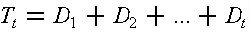

and

(6.12)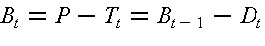

The depreciation methods most commonly used to compute Dt and Bt are the straight line method, sum-of-the-years'-digits methods, and the double declining balanced method. The U.S. Internal Revenue Service provides tables of acceptable depreciable schedules using these methods. Under straight line depreciation, the net depreciable value resulting from the cost of the facility less salvage value is allocated uniformly to each year of the estimated useful life. Under the sum-of-the-year's-digits (SOYD) method, the annual depreciation allowance is obtained by multiplying the net depreciable value multiplied by a fraction, which has as its numerator the number of years of remaining useful life and its denominator the sum of all the digits from 1 to n. The annual depreciation allowance under the double declining balance method is obtained by multiplying the book value of the previous year by a constant depreciation rate 2/n.

To consider tax effects in project evaluation, the most direct approach is to estimate the after-tax cash flow and then apply an evaluation method such as the net present value method. Since projects are often financed by internal funds representing the overall equity-debt mix of the entire corporation, the deductibility of interest on debt may be considered on a corporate-wide basis. For specific project financing from internal funds, let after-tax cash flow in year t be Yt. Then, for t=0,1,2,...,n,

(6.13)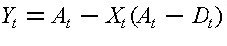

where At is the net revenue before tax in year t, Dt is the depreciation allowable for year t and Xt is the marginal corporate income tax rate in year t.

Besides corporate income taxes, there are other provisions in the federal income tax laws that affect facility investments, such as tax credits for low-income housing. Since the tax laws are revised periodically, the estimation of tax liability in the future can only be approximate.

Example 6-2: Effects of Taxes on Investment

A company plans to invest $55,000 in a piece of equipment which is expected to produce a uniform annual net revenue before tax of $15,000 over the next five years. The equipment has a salvage value of $5,000 at the end of 5 years and the depreciation allowance is computed on the basis of the straight line depreciation method. The marginal income tax rate for this company is 34%, and there is no expectation of inflation. If the after-tax MARR specified by the company is 8%, determine whether the proposed investment is worthwhile, assuming that the investment will be financed by internal funds.

Using Equations (6.11) and (6.13), the after-tax cash flow can be computed as shown in Table 6-2. Then, the net present value discounted at 8% is obtained from Equation (6.5) as follows:

The positive result indicates that the project is worthwhile.

TABLE 6-2  After-Tax Cash Flow Computation

6.8 Price Level Changes: Inflation and Deflation

In the economic evaluation of investment proposals, two approaches may be used to reflect the effects of future price level changes due to inflation or deflation. The differences between the two approaches are primarily philosophical and can be succinctly stated as follows:

1. The constant dollar approach. The investor wants a specified MARR excluding inflation. Consequently, the cash flows should be expressed in terms of base-year or constant dollars, and a discount rate excluding inflation should be used in computing the net present value.
2. The inflated dollar approach. The investor includes an inflation component in the specified MARR. Hence, the cash flows should be expressed in terms of then-current or inflated dollars, and a discount rate including inflation should be used in computing the net present value.

If these approaches are applied correctly, they will lead to identical results.

Let i be the discount rate excluding inflation, i' be the discount rate including inflation, and j be the annual inflation rate. Then,

(6.14)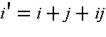

and

(6.15)

When the inflation rate j is small, these relations can be approximated by

(6.16)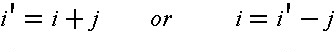

Note that inflation over time has a compounding effect on the price levels in various periods, as discussed in connection with the cost indices in Chapter 5.

If At denotes the cash flow in year t expressed in terms of constant (base year) dollars, and A't denotes the cash flow in year t expressed in terms of inflated (then-current) dollars, then

(6.17)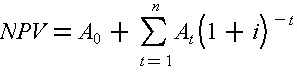

or

(6.18)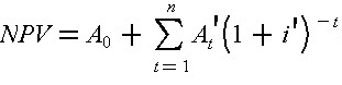

It can be shown that the results from these two equations are identical. Furthermore, the relationship applies to after-tax cash flow as well as to before-tax cash flow by replacing At and A't with Yt and Y't respectively in Equations (6.17) and (6.18).

Example 6-3: Effects of Inflation

Suppose that, in the previous example, the inflation expectation is 5% per year, and the after-tax MARR specified by the company is 8% excluding inflation. Determine whether the investment is worthwhile.

In this case, the before-tax cash flow At in terms of constant dollars at base year 0 is inflated at j = 5% to then-current dollars A't for the computation of the taxable income (A't - Dt) and income taxes. The resulting after-tax flow Y't in terms of then-current dollars is converted back to constant dollars. That is, for Xt = 34% and Dt = $10,000. The annual depreciation charges Dt are not inflated to current dollars in conformity with the practice recommended by the U.S. Internal Revenue Service. Thus:

A't = At(1 + j)t = At(1 + 0.05)t
Y't = A't - Xt(A't - Dt) = A't - (34%)(A't - $10,000)
Yt = Y't(1 + j)t = Y't(1 + 0.05)t

The detailed computation of the after-tax cash flow is recorded in Table 6-3. The net present value discounted at 8% excluding inflation is obtained by substituting Yt for At in Eq. (6.17). Hence,

[NPV]8%) = -55,000 + (13,138)(P|F, 8%, 1) + (12,985)(P|F, 8%, 2) + (12,837)(P|F, 8%, 3)
+ (12,697)(P|F, 8%, 4) + (12,564 + 5,000)(P|F, 8%, 5) = -$227

With 5% inflation, the investment is no longer worthwhile because the value of the depreciation tax deduction is not increased to match the inflation rate.

TABLE 6-3  After-Tax Cash Flow Including Inflation

Note:  B-Tax CF refers to Before-Tax Cash Flow;
           A-Tax CF refers to After-Tax Cash Flow

Example 6-4: Inflation and the Boston Central Artery Project

The cost of major construction projects are often reported as simply the sum of all expenses, no matter what year the cost was incurred. For projects extending over a lengthy period of time, this practice can combine amounts of considerably different inherent values. A good example is the Boston Central Artery/Tunnel Project, a very large project to construct or re-locate two Interstate highways within the city of Boston.

In Table 6-4, we show one estimate of the annual expenditures for the Central Artery/Tunnel from 1986 to 2006 in millions of dollars, appearing in the column labelled "Expenses ($ M)." We also show estimates of construction price inflation in the Boston area for the same period, one based on 1982 dollars (so the price index equals 100 in 1982) and one on 2002 dollars. If the dollar expenditures are added up, the total project cost is $ 14.6 Billion dollars, which is how the project cost is often reported in summary documents. However, if the cost is calculated in constant 1982 dollars (when the original project cost estimate was developed for planning purposes), the project cost would be only $ 8.4 Billion, with price inflation increasing expenses by $ 6.3 Billion. As with cost indices discussed in Chapter 5, the conversion to 1982 $ is accomplished by dividing by the 1982 price index for that year and then multiplying by 100 (the 1982 price index value). If the cost is calculated in constant 2002 dollars, the project cost increases to $ 15.8 Billion. When costs are incurred can significantly affect project expenses!

TABLE 6-4  Cash Flows for the Boston Central Artery/Tunnel Project

6.9 Uncertainty and Risk

Since future events are always uncertain, all estimates of costs and benefits used in economic evaluation involve a degree of uncertainty. Probabilistic methods are often used in decision analysis to determine expected costs and benefits as well as to assess the degree of risk in particular projects.

In estimating benefits and costs, it is common to attempt to obtain the expected or average values of these quantities depending upon the different events which might occur. Statistical techniques such as regression models can be used directly in this regard to provide forecasts of average values. Alternatively, the benefits and costs associated with different events can be estimated and the expected benefits and costs calculated as the sum over all possible events of the resulting benefits and costs multiplied by the probability of occurrence of a particular event:

(6.19)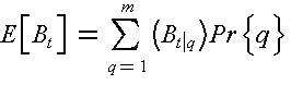

and

(6.20)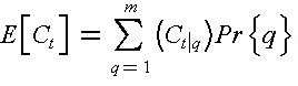

where q = 1,....,m represents possible events, (Bt|q) and (Ct|q) are benefits and costs respectively in period t due to the occurrence of q, Pr{q} is the probability that q occurs, and E[Bt] and E[Ct] are respectively expected benefit and cost in period t. Hence, the expected net benefit in period t is given by:

(6.21)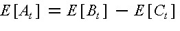

For example, the average cost of a facility in an earthquake prone site might be calculated as the sum of the cost of operation under normal conditions (multiplied by the probability of no earthquake) plus the cost of operation after an earthquake (multiplied by the probability of an earthquake). Expected benefits and costs can be used directly in the cash flow calculations described earlier.

In formulating objectives, some organizations wish to avoid risk so as to avoid the possibility of losses. In effect, a risk avoiding organization might select a project with lower expected profit or net social benefit as long as it had a lower risk of losses. This preference results in a risk premium or higher desired profit for risky projects. A rough method of representing a risk premium is to make the desired MARR higher for risky projects. Let rf be the risk free market rate of interest as represented by the average rate of return of a safe investment such as U.S. government bonds. However, U.S. government bonds do not protect from inflationary changes or exchange rate fluctuations, but only insure that the principal and interest will be repaid. Let rp be the risk premium reflecting an adjustment of the rate of return for the perceived risk. Then, the risk-adjusted rate of return r is given by:

(6.22)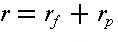

In using the risk-adjusted rate of return r to compute the net present value of an estimated net cash flow At (t = 0, 1, 2, ..., n) over n years, it is tacitly assumed that the values of At become more uncertain as time goes on. That is:

(6.23)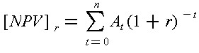

More directly, a decision maker may be confronted with the subject choice among alternatives with different expected benefits of levels of risk such that at a given period t, the decision maker is willing to exchange an uncertain At with a smaller but certain return atAt where at is less than one. Consider the decision tree in Figure 6-2 in which the decision maker is confronted with a choice between the certain return of atAt and a gamble with possible outcomes (At;)q and respective probabilities Pr{q} for q = 1,2,...,m. Then, the net present value for the series of "certainty equivalents" over n years may be computed on the basis of the risk free rate. Hence:

(6.24)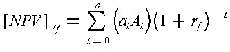

Note that if rfrp is negligible in comparison with r, then

(1 + rf)(1 + rp) = 1 +rf + rp + rfrp = 1 + r

At(1 + r)-t = (atAt/at)(1 + rf)-t(1 + rp)-t =[(atAt)(1 + rf)-t][(1 + rp)-t/at]

If at = (1 + rp)-t for t = 1,2,...,n, then Eqs. (6.23) and (6.24) will be identical. Hence, the use of the risk-adjusted rate r for computing NPV has the same effect as accepting at = (1 + rp)-t as a "certainty equivalent" factor in adjusting the estimated cash flow over time.

Figure 6-2  Determination of a Certainty Equivalent Value

6.10 Effects of Financing on Project Selection

Selection of the best design and financing plans for capital projects is typically done separately and sequentially. Three approaches to facility investment planning most often adopted by an organization are:

1. Need or demand driven: Public capital investments are defined and debated in terms of an absolute "need" for particular facilities or services. With a pre-defined "need," design and financing analysis then proceed separately. Even when investments are made on the basis of a demand or revenue analysis of the market, the separation of design and financing analysis is still prevalent.
2. Design driven: Designs are generated, analyzed and approved prior to the investigation of financing alternatives, because projects are approved first and only then programmed for eventual funding.
3. Finance driven: The process of developing a facility within a particular budget target is finance-driven since the budget is formulated prior to the final design. It is a common procedure in private developments and increasingly used for public projects.

Typically, different individuals or divisions of an organization conduct the analysis for the operating and financing processes. Financing alternatives are sometimes not examined at all since a single mechanism is universally adopted. An example of a single financing plan in the public sector is the use of pay-as-you-go highway trust funds. However, the importance of financial analysis is increasing with the increase of private ownership and private participation in the financing of public projects. The availability of a broad spectrum of new financing instruments has accentuated the needs for better financial analysis in connection with capital investments in both the public and private sectors. While simultaneous assessment of all design and financing alternatives is not always essential, more communication of information between the two evaluation processes would be advantageous in order to avoid the selection of inferior alternatives.

There is an ever increasing variety of borrowing mechanisms available. First, the extent to which borrowing is tied to a particular project or asset may be varied. Loans backed by specific, tangible and fungible assets and with restrictions on that asset's use are regarded as less risky. In contrast, specific project finance may be more costly to arrange due to transactions costs than is general corporate or government borrowing. Also, backing by the full good faith and credit of an organization is considered less risky than investments backed by generally immovable assets. Second, the options of fixed versus variable rate borrowing are available. Third, the repayment schedule and time horizon of borrowing may be varied. A detailed discussion of financing of constructed facilities will be deferred until the next chapter.

As a general rule, it is advisable to borrow as little as possible when borrowing rates exceed the minimum attractive rate of return. Equity or pay-as-you-go financing may be desirable in this case. It is generally preferable to obtain lower borrowing rates, unless borrowing associated with lower rates requires substantial transaction costs or reduces the flexibility for repayment and refinancing. In the public sector, it may be that increasing taxes or user charges to reduce borrowing involves economic costs in excess of the benefits of reduced borrowing costs of borrowed funds. Furthermore, since cash flow analysis is typically conducted on the basis of constant dollars and loan agreements are made with respect to current dollars, removing the effects of inflation will reduce the cost of borrowing. Finally, deferring investments until pay-as-you-go or equity financing are available may unduly defer the benefits of new investments.

It is difficult to conclude unambiguously that one financing mechanism is always superior to others. Consequently, evaluating alternative financing mechanisms is an important component of the investment analysis procedure. One possible approach to simultaneously considering design and financing alternatives is to consider each combination of design and financing options as a specific, mutually exclusive alternative. The cash flow of this combined alternative would be the sum of the economic or operating cash flow (assuming equity financing) and the financial cash flow over the planning horizon.

6.11 Combined Effects of Operating and Financing Cash Flows

A general approach for obtaining the combined effects of operating and financing cash flows of a project is to make use of the additive property of net present values by calculating an adjusted net present value. The adjusted net present value (APV) is the sum of the net present value (NPV) of the operating cash flow plus the net present value of the financial cash flow due to borrowing or raising capital (FPV). Thus,

(6.25)

where each function is evaluated at i=MARR if both the operating and the financing cash flows have the same degree of risk or if the risks are taken care of in other ways such as by the use of certainty equivalents. Then, project selection involving both design and financing alternatives is accomplished by selecting the combination which has the highest positive adjusted present value. The use of this adjusted net present value method will result in the same selection as an evaluation based on the net present value obtained from the combined cash flow of each alternative combination directly.

To be specific, let At be the net operating cash flow, be the net financial cash flow resulting from debt financing, and AAt be the combined net cash flow, all for year t before tax. Then:

(6.26)

Similarly, let and YYt be the corresponding cash flows after tax such that:

(6.27)

The tax shields for interest on borrowing (for t = 1, 2, ..., n) are usually given by

(6.28)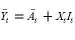

where It is the interest paid in year t and Xt is the marginal corporate income tax rate in year t. In view of Eqs. (6.13), (6.27) and (6.28), we obtain

(6.29)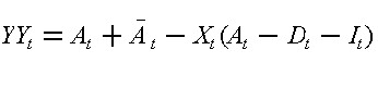

When MARR = i is applied to both the operating and the financial cash flows in Eqs. (6.13) and (6.28), respectively, in computing the net present values, the combined effect will be the same as the net present value obtained by applying MARR = i to the combined cash flow in Eq. (6.29).

In many instances, a risk premium related to the specified type of operation is added to the MARR for discounting the operating cash flow. On the other hand, the MARR for discounting the financial cash flow for borrowing is often regarded as relatively risk-free because debtors or holders of corporate bonds must be paid first before stockholders in case financial difficulties are encountered by a corporation. Then, the adjusted net present value is given by

(6.30)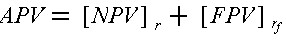

where NPV is discounted at r and FPV is obtained from the rf rate. Note that the net present value of the financial cash flow includes not only tax shields for interest on loans and other forms of government subsidy, but also on transactions costs such as those for legal and financial services associated with issuing new bonds or stocks.

The evaluation of combined alternatives based on the adjusted net present value method should also be performed in dollar amounts which either consistently include or remove the effects of inflation. The MARR value used would reflect the inclusion or exclusion of inflation accordingly. Furthermore, it is preferable to use after-tax cash flows in the evaluation of projects for private firms since different designs and financing alternatives are likely to have quite different implications for tax liabilities and tax shields.

In theory, the corporate finance process does not necessarily require a different approach than that of the APV method discussed above. Rather than considering single projects in isolation, groups or sets of projects along with financing alternatives can be evaluated. The evaluation process would be to select that group of operating and financing plans which has the highest total APV. Unfortunately, the number of possible combinations to evaluate can become very large even though many combinations can be rapidly eliminated in practice because they are clearly inferior. More commonly, heuristic approaches are developed such as choosing projects with the highest benefit/cost ratio within a particular budget or financial constraint. These heuristic schemes will often involve the separation of the financing and design alternative evaluation. The typical result is design-driven or finance-driven planning in which one or the other process is conducted first.

Example 6-5: Combined Effects of Operating and Financing Plans

A public agency plans to construct a facility and is considering two design alternatives with different capacities. The operating net cash flows for both alternatives over a planning horizon of 5 years are shown in Table 6-4. For each design alternative, the project can be financed either through overdraft on bank credit or by issuing bonds spanning over the 5-year period, and the cash flow for each financing alternative is also shown in Table 6-4. The public agency has specified a MARR of 10% for discounting the operating and financing cash flows for this project. Determine the best combination of design and financing plan if

(a) a design is selected before financing plans are considered, or
(b) the decision is made simultaneously rather than sequentially.

The net present values (NPV) of all cash flows can be computed by Eq.(6.5), and the results are given at the bottom of Table 6-4. The adjusted net present value (APV) combining the operating cash flow of each design and an appropriate financing is obtained according to Eq. (6.25), and the results are also tabulated at the bottom of Table 6-4.

Under condition (a), design alternative 2 will be selected since NPV = $767,000 is the higher value when only operating cash flows are considered. Subsequently, bonds financing will be chosen because APV = $466,000 indicates that it is the best financing plan for design alternative 2.

Under condition (b), however, the choice will be based on the highest value of APV, i.e., APV = $484,000 for design alternative one in combination will overdraft financing. Thus, the simultaneous decision approach will yield the best results.

TABLE 6-5  Illustration of Different Design and Financing Alternatives (in $ thousands)