11.3 Calculations for Monte Carlo Schedule Simulation

In this section, we outline the procedures required to perform Monte Carlo simulation for the purpose of schedule analysis. These procedures presume that the various steps involved in forming a network plan and estimating the characteristics of the probability distributions for the various activities have been completed. Given a plan and the activity duration distributions, the heart of the Monte Carlo simulation procedure is the derivation of a realization or synthetic outcome of the relevant activity durations. Once these realizations are generated, standard scheduling techniques can be applied. We shall present the formulas associated with the generation of normally distributed activity durations, and then comment on the requirements for other distributions in an example.

To generate normally distributed realizations of activity durations, we can use a two step procedure. First, we generate uniformly distributed random variables, ui in the interval from zero to one. Numerous techniques can be used for this purpose. For example, a general formula for random number generation can be of the form:

(11.6)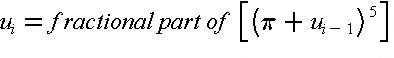

where = 3.14159265 and ui-1 was the previously generated random number or a pre-selected beginning or seed number. For example, a seed of u0 = 0.215 in Eq. (11.6) results in u1 = 0.0820, and by applying this value of u1, the result is u2 = 0.1029. This formula is a special case of the mixed congruential method of random number generation. While Equation (11.6) will result in a series of numbers that have the appearance and the necessary statistical properties of true random numbers, we should note that these are actually "pseudo" random numbers since the sequence of numbers will repeat given a long enough time.

With a method of generating uniformly distributed random numbers, we can generate normally distributed random numbers using two uniformly distributed realizations with the equations:

(11.7)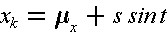

with

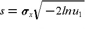
where xk is the normal realization, x is the mean of x, x is the standard deviation of x, and u1 and u2 are the two uniformly distributed random variable realizations. For the case in which the mean of an activity is 2.5 days and the standard deviation of the duration is 1.5 days, a corresponding realization of the duration is s = 2.2365, t = 0.6465 and xk = 2.525 days, using the two uniform random numbers generated from a seed of 0.215 above.

Correlated random number realizations may be generated making use of conditional distributions. For example, suppose that the duration of an activity d is normally distributed and correlated with a second normally distributed random variable x which may be another activity duration or a separate factor such as a weather effect. Given a realization xk of x, the conditional distribution of d is still normal, but it is a function of the value xk. In particular, the conditional mean ('d|x = xk) and standard deviation ('d|x = xk) of a normally distributed variable given a realization of the second variable is:

(11.8)

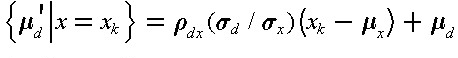
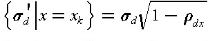
where dx is the correlation coefficient between d and x. Once xk is known, the conditional mean and standard deviation can be calculated from Eq. (11.8) and then a realization of d obtained by applying Equation (11.7).

Correlation coefficients indicate the extent to which two random variables will tend to vary together. Positive correlation coefficients indicate one random variable will tend to exceed its mean when the other random variable does the same. From a set of n historical observations of two random variables, x and y, the correlation coefficient can be estimated as:

(11.9)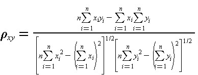

The value of xy can range from one to minus one, with values near one indicating a positive, near linear relationship between the two random variables.

It is also possible to develop formulas for the conditional distribution of a random variable correlated with numerous other variables; this is termed a multi-variate distribution. Random number generations from other types of distributions are also possible. Once a set of random variable distributions is obtained, then the process of applying a scheduling algorithm is required as described in previous sections.

Example 11-2: A Three-Activity Project Example

Suppose that we wish to apply a Monte Carlo simulation procedure to a simple project involving three activities in series. As a result, the critical path for the project includes all three activities. We assume that the durations of the activities are normally distributed with the following parameters:

Activity	Mean (Days)	Standard Deviation (Days)
A B C	2.5 5.6 2.4	1.5 2.4 2.0

To simulate the schedule effects, we generate the duration realizations shown in Table 11-3 and calculate the project duration for each set of three activity duration realizations.

For the twelve sets of realizations shown in the table, the mean and standard deviation of the project duration can be estimated to be 10.49 days and 4.06 days respectively. In this simple case, we can also obtain an analytic solution for this duration, since it is only the sum of three independent normally distributed variables. The actual project duration has a mean of 10.5 days, and a standard deviation of days. With only a limited number of simulations, the mean obtained from simulations is close to the actual mean, while the estimated standard deviation from the simulation differs significantly from the actual value. This latter difference can be attributed to the nature of the set of realizations used in the simulations; using a larger number of simulated durations would result in a more accurate estimate of the standard deviation.

TABLE 11-3  Duration Realizations for a Monte Carlo Schedule Simulation

Example 11-3: Generation of Realizations from Triangular Distributions

To simplify calculations for Monte Carlo simulation of schedules, the use of a triangular distribution is advantageous compared to the normal or the beta distributions. Triangular distributions also have the advantage relative to the normal distribution that negative durations cannot be estimated. As illustrated in Figure 11-2, the triangular distribution can be skewed to the right or left and has finite limits like the beta distribution. If a is the lower limit, b the upper limit and m the most likely value, then the mean and standard deviation of a triangular distribution are:

(11.10)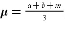

(11.11)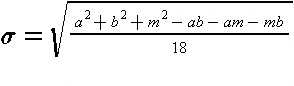

The cumulative probability function for the triangular distribution is:

(11.12)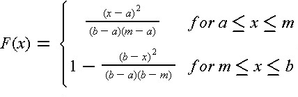

where F(x) is the probability that the random variable is less than or equal to the value of x.

Figure 11-2  Illustration of Two Triangular Activity Duration Distributions

Generating a random variable from this distribution can be accomplished with a single uniform random variable realization using the inversion method. In this method, a realization of the cumulative probability function, F(x) is generated and the corresponding value of x is calculated. Since the cumulative probability function varies from zero to one, the density function realization can be obtained from the uniform value random number generator, Equation (11.6). The calculation of the corresponding value of x is obtained from inverting Equation (11.12):

(11.13)

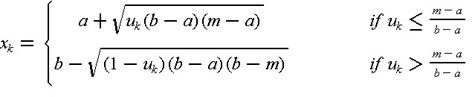
For example, if a = 3.2, m = 4.5 and b = 6.0, then x = 4.8 and x = 2.7. With a uniform realization of u = 0.215, then for (m-a)/(b-a) 0.215, x will lie between a and m and is found to have a value of 4.1 from Equation (11.13).