13.5 Quality Control by Statistical Methods

An ideal quality control program might test all materials and work on a particular facility. For example, non-destructive techniques such as x-ray inspection of welds can be used throughout a facility. An on-site inspector can witness the appropriateness and adequacy of construction methods at all times. Even better, individual craftsmen can perform continuing inspection of materials and their own work. Exhaustive or 100% testing of all materials and work by inspectors can be exceedingly expensive, however. In many instances, testing requires the destruction of a material sample, so exhaustive testing is not even possible. As a result, small samples are used to establish the basis of accepting or rejecting a particular work item or shipment of materials. Statistical methods are used to interpret the results of test on a small sample to reach a conclusion concerning the acceptability of an entire lot or batch of materials or work products.

The use of statistics is essential in interpreting the results of testing on a small sample. Without adequate interpretation, small sample testing results can be quite misleading. As an example, suppose that there are ten defective pieces of material in a lot of one hundred. In taking a sample of five pieces, the inspector might not find any defective pieces or might have all sample pieces defective. Drawing a direct inference that none or all pieces in the population are defective on the basis of these samples would be incorrect. Due to this random nature of the sample selection process, testing results can vary substantially. It is only with statistical methods that issues such as the chance of different levels of defective items in the full lot can be fully analyzed from a small sample test.

There are two types of statistical sampling which are commonly used for the purpose of quality control in batches of work or materials:

1. The acceptance or rejection of a lot is based on the number of defective (bad) or nondefective (good) items in the sample. This is referred to as sampling by attributes.
2. Instead of using defective and nondefective classifications for an item, a quantitative quality measure or the value of a measured variable is used as a quality indicator. This testing procedure is referred to as sampling by variables.

Whatever sampling plan is used in testing, it is always assumed that the samples are representative of the entire population under consideration. Samples are expected to be chosen randomly so that each member of the population is equally likely to be chosen. Convenient sampling plans such as sampling every twentieth piece, choosing a sample every two hours, or picking the top piece on a delivery truck may be adequate to insure a random sample if pieces are randomly mixed in a stack or in use. However, some convenient sampling plans can be inappropriate. For example, checking only easily accessible joints in a building component is inappropriate since joints that are hard to reach may be more likely to have erection or fabrication problems.

Another assumption implicit in statistical quality control procedures is that the quality of materials or work is expected to vary from one piece to another. This is certainly true in the field of construction. While a designer may assume that all concrete is exactly the same in a building, the variations in material properties, manufacturing, handling, pouring, and temperature during setting insure that concrete is actually heterogeneous in quality. Reducing such variations to a minimum is one aspect of quality construction. Insuring that the materials actually placed achieve some minimum quality level with respect to average properties or fraction of defectives is the task of quality control.

13.6 Statistical Quality Control with Sampling by Attributes

Sampling by attributes is a widely applied quality control method. The procedure is intended to determine whether or not a particular group of materials or work products is acceptable. In the literature of statistical quality control, a group of materials or work items to be tested is called a lot or batch. An assumption in the procedure is that each item in a batch can be tested and classified as either acceptable or deficient based upon mutually acceptable testing procedures and acceptance criteria. Each lot is tested to determine if it satisfies a minimum acceptable quality level (AQL) expressed as the maximum percentage of defective items in a lot or process.

In its basic form, sampling by attributes is applied by testing a pre-defined number of sample items from a lot. If the number of defective items is greater than a trigger level, then the lot is rejected as being likely to be of unacceptable quality. Otherwise, the lot is accepted. Developing this type of sampling plan requires consideration of probability, statistics and acceptable risk levels on the part of the supplier and consumer of the lot. Refinements to this basic application procedure are also possible. For example, if the number of defectives is greater than some pre-defined number, then additional sampling may be started rather than immediate rejection of the lot. In many cases, the trigger level is a single defective item in the sample. In the remainder of this section, the mathematical basis for interpreting this type of sampling plan is developed.

More formally, a lot is defined as acceptable if it contains a fraction p1 or less defective items. Similarly, a lot is defined as unacceptable if it contains a fraction p2 or more defective units. Generally, the acceptance fraction is less than or equal to the rejection fraction, p1 p2, and the two fractions are often equal so that there is no ambiguous range of lot acceptability between p1 and p2. Given a sample size and a trigger level for lot rejection or acceptance, we would like to determine the probabilities that acceptable lots might be incorrectly rejected (termed producer's risk) or that deficient lots might be incorrectly accepted (termed consumer's risk).

Consider a lot of finite number N, in which m items are defective (bad) and the remaining (N-m) items are non-defective (good). If a random sample of n items is taken from this lot, then we can determine the probability of having different numbers of defective items in the sample. With a pre-defined acceptable number of defective items, we can then develop the probability of accepting a lot as a function of the sample size, the allowable number of defective items, and the actual fraction of defective items. This derivation appears below.

The number of different samples of size n that can be selected from a finite population N is termed a mathematical combination and is computed as:

(13.1)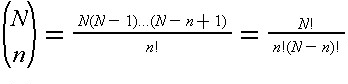

where a factorial, n! is n*(n-1)*(n-2)...(1) and zero factorial (0!) is one by convention. The number of possible samples with exactly x defectives is the combination associated with obtaining x defectives from m possible defective items and n-x good items from N-m good items:

(13.2)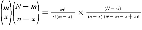

Given these possible numbers of samples, the probability of having exactly x defective items in the sample is given by the ratio as the hypergeometric series:

(13.3)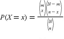

With this function, we can calculate the probability of obtaining different numbers of defectives in a sample of a given size.

Suppose that the actual fraction of defectives in the lot is p and the actual fraction of nondefectives is q, then p plus q is one, resulting in m = Np, and N - m = Nq. Then, a function g(p) representing the probability of having r or less defective items in a sample of size n is obtained by substituting m and N into Eq. (13.3) and summing over the acceptable defective number of items:

(13.4)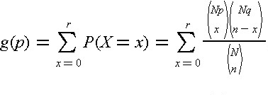

If the number of items in the lot, N, is large in comparison with the sample size n, then the function g(p) can be approximated by the binomial distribution:

(13.5)

or

(13.6)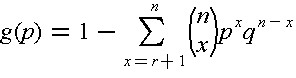

The function g(p) indicates the probability of accepting a lot, given the sample size n and the number of allowable defective items in the sample r. The function g(p) can be represented graphical for each combination of sample size n and number of allowable defective items r, as shown in Figure 13-1. Each curve is referred to as the operating characteristic curve (OC curve) in this graph. For the special case of a single sample (n=1), the function g(p) can be simplified:

(13.7)

so that the probability of accepting a lot is equal to the fraction of acceptable items in the lot. For example, there is a probability of 0.5 that the lot may be accepted from a single sample test even if fifty percent of the lot is defective.

Figure 13-1  Example Operating Characteristic Curves Indicating Probability of Lot Acceptance

For any combination of n and r, we can read off the value of g(p) for a given p from the corresponding OC curve. For example, n = 15 is specified in Figure 13-1. Then, for various values of r, we find:

The producer's and consumer's risk can be related to various points on an operating characteristic curve. Producer's risk is the chance that otherwise acceptable lots fail the sampling plan (ie. have more than the allowable number of defective items in the sample) solely due to random fluctuations in the selection of the sample. In contrast, consumer's risk is the chance that an unacceptable lot is acceptable (ie. has less than the allowable number of defective items in the sample) due to a better than average quality in the sample. For example, suppose that a sample size of 15 is chosen with a trigger level for rejection of one item. With a four percent acceptable level and a greater than four percent defective fraction, the consumer's risk is at most eighty-eight percent. In contrast, with a four percent acceptable level and a four percent defective fraction, the producer's risk is at most 1 - 0.88 = 0.12 or twelve percent.

In specifying the sampling plan implicit in the operating characteristic curve, the supplier and consumer of materials or work must agree on the levels of risk acceptable to themselves. If the lot is of acceptable quality, the supplier would like to minimize the chance or risk that a lot is rejected solely on the basis of a lower than average quality sample. Similarly, the consumer would like to minimize the risk of accepting under the sampling plan a deficient lot. In addition, both parties presumably would like to minimize the costs and delays associated with testing. Devising an acceptable sampling plan requires trade off the objectives of risk minimization among the parties involved and the cost of testing.

Example 13-3: Acceptance probability calculation

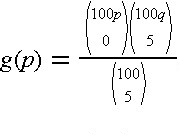
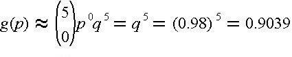
Suppose that the sample size is five (n=5) from a lot of one hundred items (N=100). The lot of materials is to be rejected if any of the five samples is defective (r = 0). In this case, the probability of acceptance as a function of the actual number of defective items can be computed by noting that for r = 0, only one term (x = 0) need be considered in Eq. (13.4). Thus, for N = 100 and n = 5:

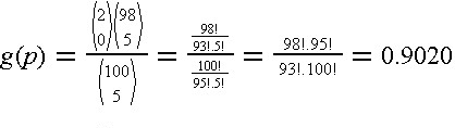
For a two percent defective fraction (p = 0.02), the resulting acceptance value is:

Using the binomial approximation in Eq. (13.5), the comparable calculation would be:

which is a difference of 0.0019, or 0.21 percent from the actual value of 0.9020 found above.

If the acceptable defective proportion was two percent (so p1 = p2 = 0.02), then the chance of an incorrect rejection (or producer's risk) is 1 - g(0.02) = 1 - 0.9 = 0.1 or ten percent. Note that a prudent producer should insure better than minimum quality products to reduce the probability or chance of rejection under this sampling plan. If the actual proportion of defectives was one percent, then the producer's risk would be only five percent with this sampling plan.

Example 13-4: Designing a Sampling Plan

Suppose that an owner (or product "consumer" in the terminology of quality control) wishes to have zero defective items in a facility with 5,000 items of a particular kind. What would be the different amounts of consumer's risk for different sampling plans?

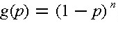
With an acceptable quality level of no defective items (so p1 = 0), the allowable defective items in the sample is zero (so r = 0) in the sampling plan. Using the binomial approximation, the probability of accepting the 5,000 items as a function of the fraction of actual defective items and the sample size is:

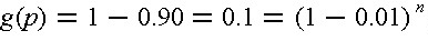
To insure a ninety percent chance of rejecting a lot with an actual percentage defective of one percent (p = 0.01), the required sample size would be calculated as:

Then,

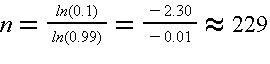
As can be seen, large sample sizes are required to insure relatively large probabilities of zero defective items.