11. Advanced Scheduling Techniques
11.1 Use of Advanced Scheduling Techniques
Construction project scheduling is a topic that has received extensive research over a number of decades. The previous chapter described the fundamental scheduling techniques widely used and supported by numerous commercial scheduling systems. A variety of special techniques have also been developed to address specific circumstances or problems. With the availability of more powerful computers and software, the use of advanced scheduling techniques is becoming easier and of greater relevance to practice. In this chapter, we survey some of the techniques that can be employed in this regard. These techniques address some important practical problems, such as:
A final section in the chapter describes some possible improvements in the project scheduling process. In Chapter 14, we consider issues of computer based implementation of scheduling procedures, particularly in the context of integrating scheduling with other project management procedures.
11.2 Scheduling with Uncertain Durations
Section 10.3 described the application of critical path scheduling for the situation in which activity durations are fixed and known. Unfortunately, activity durations are estimates of the actual time required, and there is liable to be a significant amount of uncertainty associated with the actual durations. During the preliminary planning stages for a project, the uncertainty in activity durations is particularly large since the scope and obstacles to the project are still undefined. Activities that are outside of the control of the owner are likely to be more uncertain. For example, the time required to gain regulatory approval for projects may vary tremendously. Other external events such as adverse weather, trench collapses, or labor strikes make duration estimates particularly uncertain.
Two simple approaches to dealing with the uncertainty in activity durations warrant some discussion before introducing more formal scheduling procedures to deal with uncertainty. First, the uncertainty in activity durations may simply be ignored and scheduling done using the expected or most likely time duration for each activity. Since only one duration estimate needs to be made for each activity, this approach reduces the required work in setting up the original schedule. Formal methods of introducing uncertainty into the scheduling process require more work and assumptions. While this simple approach might be defended, it has two drawbacks. First, the use of expected activity durations typically results in overly optimistic schedules for completion; a numerical example of this optimism appears below. Second, the use of single activity durations often produces a rigid, inflexible mindset on the part of schedulers. As field managers appreciate, activity durations vary considerable and can be influenced by good leadership and close attention. As a result, field managers may loose confidence in the realism of a schedule based upon fixed activity durations. Clearly, the use of fixed activity durations in setting up a schedule makes a continual process of monitoring and updating the schedule in light of actual experience imperative. Otherwise, the project schedule is rapidly outdated.
A second simple approach to incorporation uncertainty also deserves mention. Many managers recognize that the use of expected durations may result in overly optimistic schedules, so they include a contingency allowance in their estimate of activity durations. For example, an activity with an expected duration of two days might be scheduled for a period of 2.2 days, including a ten percent contingency. Systematic application of this contingency would result in a ten percent increase in the expected time to complete the project. While the use of this rule-of-thumb or heuristic contingency factor can result in more accurate schedules, it is likely that formal scheduling methods that incorporate uncertainty more formally are useful as a means of obtaining greater accuracy or in understanding the effects of activity delays.
The most common formal approach to incorporate uncertainty in the scheduling process is to apply the critical path scheduling process (as described in Section 10.3) and then analyze the results from a probabilistic perspective. This process is usually referred to as the PERT scheduling or evaluation method. As noted earlier, the duration of the critical path represents the minimum time required to complete the project. Using expected activity durations and critical path scheduling, a critical path of activities can be identified. This critical path is then used to analyze the duration of the project incorporating the uncertainty of the activity durations along the critical path. The expected project duration is equal to the sum of the expected durations of the activities along the critical path. Assuming that activity durations are independent random variables, the variance or variation in the duration of this critical path is calculated as the sum of the variances along the critical path. With the mean and variance of the identified critical path known, the distribution of activity durations can also be computed.
The mean and variance for each activity duration are typically computed from estimates of "optimistic" (ai,j), "most likely" (mi,j), and "pessimistic" (bi,j) activity durations using the formulas:
(11.1)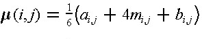
and
(11.2)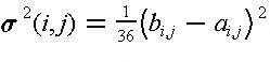
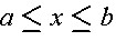
where  and and  are the mean duration and its variance, respectively, of an activity (i,j). Three activity durations estimates (i.e., optimistic, most likely, and pessimistic durations) are required in the calculation. The use of these optimistic, most likely, and pessimistic estimates stems from the fact that these are thought to be easier for managers to estimate subjectively. The formulas for calculating the mean and variance are derived by assuming that the activity durations follow a probabilistic beta distribution under a restrictive condition. The probability density function of a beta distributions for a random varable x is given by: are the mean duration and its variance, respectively, of an activity (i,j). Three activity durations estimates (i.e., optimistic, most likely, and pessimistic durations) are required in the calculation. The use of these optimistic, most likely, and pessimistic estimates stems from the fact that these are thought to be easier for managers to estimate subjectively. The formulas for calculating the mean and variance are derived by assuming that the activity durations follow a probabilistic beta distribution under a restrictive condition. The probability density function of a beta distributions for a random varable x is given by:
(11.3)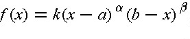
 and and 
where k is a constant which can be expressed in terms of  and and  . Several beta distributions for different sets of values of and are shown in Figure 11-1. For a beta distribution in the interval having a modal value m, the mean is given by: . Several beta distributions for different sets of values of and are shown in Figure 11-1. For a beta distribution in the interval having a modal value m, the mean is given by:
(11.4)
If + = 4, then Eq. (11.4) will result in Eq. (11.1). Thus, the use of Eqs. (11.1) and (11.2) impose an additional condition on the beta distribution. In particular, the restriction that  = (b - a)/6 is imposed. = (b - a)/6 is imposed.
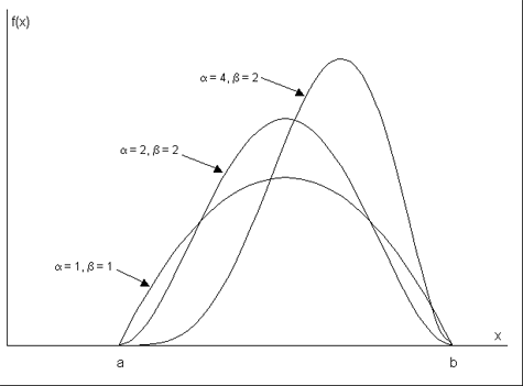
Figure 11-1 Illustration of Several Beta Distributions
Since absolute limits on the optimistic and pessimistic activity durations are extremely difficult to estimate from historical data, a common practice is to use the ninety-fifth percentile of activity durations for these points. Thus, the optimistic time would be such that there is only a one in twenty (five percent) chance that the actual duration would be less than the estimated optimistic time. Similarly, the pessimistic time is chosen so that there is only a five percent chance of exceeding this duration. Thus, there is a ninety percent chance of having the actual duration of an activity fall between the optimistic and pessimistic duration time estimates. With the use of ninety-fifth percentile values for the optimistic and pessimistic activity duration, the calculation of the expected duration according to Eq. (11.1) is unchanged but the formula for calculating the activity variance becomes:
(11.5)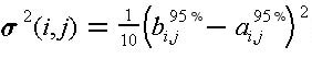
The difference between Eqs. (11.2) and (11.5) comes only in the value of the divisor, with 36 used for absolute limits and 10 used for ninety-five percentile limits. This difference might be expected since the difference between bi,j and ai,j would be larger for absolute limits than for the ninety-fifth percentile limits.
While the PERT method has been made widely available, it suffers from three major problems. First, the procedure focuses upon a single critical path, when many paths might become critical due to random fluctuations. For example, suppose that the critical path with longest expected time happened to be completed early. Unfortunately, this does not necessarily mean that the project is completed early since another path or sequence of activities might take longer. Similarly, a longer than expected duration for an activity not on the critical path might result in that activity suddenly becoming critical. As a result of the focus on only a single path, the PERT method typically underestimates the actual project duration.
As a second problem with the PERT procedure, it is incorrect to assume that most construction activity durations are independent random variables. In practice, durations are correlated with one another. For example, if problems are encountered in the delivery of concrete for a project, this problem is likely to influence the expected duration of numerous activities involving concrete pours on a project. Positive correlations of this type between activity durations imply that the PERT method underestimates the variance of the critical path and thereby produces over-optimistic expectations of the probability of meeting a particular project completion deadline.
Finally, the PERT method requires three duration estimates for each activity rather than the single estimate developed for critical path scheduling. Thus, the difficulty and labor of estimating activity characteristics is multiplied threefold.
As an alternative to the PERT procedure, a straightforward method of obtaining information about the distribution of project completion times (as well as other schedule information) is through the use of Monte Carlo simulation. This technique calculates sets of artificial (but realistic) activity duration times and then applies a deterministic scheduling procedure to each set of durations. Numerous calculations are required in this process since simulated activity durations must be calculated and the scheduling procedure applied many times. For realistic project networks, 40 to 1,000 separate sets of activity durations might be used in a single scheduling simulation. The calculations associated with Monte Carlo simulation are described in the following section.
A number of different indicators of the project schedule can be estimated from the results of a Monte Carlo simulation:
The disadvantage of Monte Carlo simulation results from the additional information about activity durations that is required and the computational effort involved in numerous scheduling applications for each set of simulated durations. For each activity, the distribution of possible durations as well as the parameters of this distribution must be specified. For example, durations might be assumed or estimated to be uniformly distributed between a lower and upper value. In addition, correlations between activity durations should be specified. For example, if two activities involve assembling forms in different locations and at different times for a project, then the time required for each activity is likely to be closely related. If the forms pose some problems, then assembling them on both occasions might take longer than expected. This is an example of a positive correlation in activity times. In application, such correlations are commonly ignored, leading to errors in results. As a final problem and discouragement, easy to use software systems for Monte Carlo simulation of project schedules are not generally available. This is particularly the case when correlations between activity durations are desired.
Another approach to the simulation of different activity durations is to develop specific scenarios of events and determine the effect on the overall project schedule. This is a type of "what-if" problem solving in which a manager simulates events that might occur and sees the result. For example, the effects of different weather patterns on activity durations could be estimated and the resulting schedules for the different weather patterns compared. One method of obtaining information about the range of possible schedules is to apply the scheduling procedure using all optimistic, all most likely, and then all pessimistic activity durations. The result is three project schedules representing a range of possible outcomes. This process of "what-if" analysis is similar to that undertaken during the process of construction planning or during analysis of project crashing.
Example 11-1: Scheduling activities with uncertain time durations.
Suppose that the nine activity example project shown in Table 10-2 and Figure 10-4 of Chapter 10 was thought to have very uncertain activity time durations. As a result, project scheduling considering this uncertainty is desired. All three methods (PERT, Monte Carlo simulation, and "What-if" simulation) will be applied.
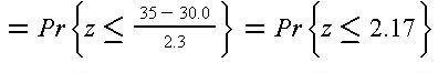
Table 11-1 shows the estimated optimistic, most likely and pessimistic durations for the nine activities. From these estimates, the mean, variance and standard deviation are calculated. In this calculation, ninety-fifth percentile estimates of optimistic and pessimistic duration times are assumed, so that Equation (11.5) is applied. The critical path for this project ignoring uncertainty in activity durations consists of activities A, C, F and I as found in Table 10-3 (Section 10.3). Applying the PERT analysis procedure suggests that the duration of the project would be approximately normally distributed. The sum of the means for the critical activities is 4.0 + 8.0 + 12.0 + 6.0 = 30.0 days, and the sum of the variances is 0.4 + 1.6 + 1.6 + 1.6 = 5.2 leading to a standard deviation of 2.3 days.
With a normally distributed project duration, the probability of meeting a project deadline is equal to the probability that the standard normal distribution is less than or equal to (PD -  D)|D where PD is the project deadline, D is the expected duration and D is the standard deviation of project duration. For example, the probability of project completion within 35 days is: D)|D where PD is the project deadline, D is the expected duration and D is the standard deviation of project duration. For example, the probability of project completion within 35 days is:
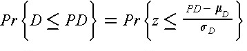
where z is the standard normal distribution tabulated value of the cumulative standard distribution appears in Table B.1 of Appendix B.
Monte Carlo simulation results provide slightly different estimates of the project duration characteristics. Assuming that activity durations are independent and approximately normally distributed random variables with the mean and variances shown in Table 11-1, a simulation can be performed by obtaining simulated duration realization for each of the nine activities and applying critical path scheduling to the resulting network. Applying this procedure 500 times, the average project duration is found to be 30.9 days with a standard deviation of 2.5 days. The PERT result is less than this estimate by 0.9 days or three percent. Also, the critical path considered in the PERT procedure (consisting of activities A, C, F and I) is found to be the critical path in the simulated networks less than half the time.
TABLE 11-1 Activity Duration Estimates for a Nine Activity Project
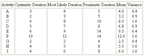
If there are correlations among the activity durations, then significantly different results can be obtained. For example, suppose that activities C, E, G and H are all positively correlated random variables with a correlation of 0.5 for each pair of variables. Applying Monte Carlo simulation using 500 activity network simulations results in an average project duration of 36.5 days and a standard deviation of 4.9 days. This estimated average duration is 6.5 days or 20 percent longer than the PERT estimate or the estimate obtained ignoring uncertainty in durations. If correlations like this exist, these methods can seriously underestimate the actual project duration.
Finally, the project durations obtained by assuming all optimistic and all pessimistic activity durations are 23 and 41 days respectively. Other "what-if" simulations might be conducted for cases in which peculiar soil characteristics might make excavation difficult; these soil peculiarities might be responsible for the correlations of excavation activity durations described above.
Results from the different methods are summarized in Table 11-2. Note that positive correlations among some activity durations results in relatively large increases in the expected project duration and variability.
TABLE 11-2 Project Duration Results from Various Techniques and Assumptions for an Example
|
