10.7 Calculations for Scheduling with Leads, Lags and Windows
Table 10-9 contains an algorithmic description of the calculations required for critical path scheduling with leads, lags and windows. This description assumes an activity-on-node project network representation, since this representation is much easier to use with complicated precedence relationships. The possible precedence relationships accomadated by the procedure contained in Table 10-9 are finish-to-start leads, start-to-start leads, finish-to-finish lags and start-to-finish lags. Windows for earliest starts or latest finishes are also accomodated. Incorporating other precedence and window types in a scheduling procedure is also possible as described in Chapter 11. With an activity-on-node representation, we assume that an initiation and a termination activity are included to mark the beginning and end of the project. The set of procedures described in Table 10-9 does not provide for automatic splitting of activities.
TABLE 10-9 Critical Path Scheduling Algorithms with Leads, Lags and Windows (Activity-on-Node Representations)
The first step in the scheduling algorithm is to sort activities such that no higher numbered activity precedes a lower numbered activity. With numbered activities, durations can be denoted D(k), where k is the number of an activity. Other activity information can also be referenced by the activity number. Note that node events used in activity-on-branch representations are not required in this case.
The forward pass calculations compute an earliest start time (ES(k)) and an earliest finish time (EF(k)) for each activity in turn (Table 10-9). In computing the earliest start time of an activity k, the earliest start window time (WES), the earliest finish window time (WEF), and each of the various precedence relationships must be considered. Constraints on finish times are included by identifying minimum finish times and then subtracting the activity duration. A default earliest start time of day 0 is also insured for all activities. A second step in the procedure is to identify each activity's earliest finish time (EF(k)).
The backward pass calculations proceed in a manner very similar to those of the forward pass (Table 10-9). In the backward pass, the latest finish and the latest start times for each activity are calculated. In computing the latest finish time, the latest start time is identified which is consistent with precedence constraints on an activity's starting time. This computation requires a minimization over applicable window times and all successor activities. A check for a feasible activity schedule can also be imposed at this point: if the late start time is less than the early start time (LS(k) < ES(k)), then the activity schedule is not possible.
The result of the forward and backward pass calculations are the earliest start time, the latest start time, the earliest finish time, and the latest finish time for each activity. The activity float is computed as the latest start time less the earliest start time. Note that window constraints may be instrumental in setting the amount of float, so that activities without any float may either lie on the critical path or be constrained by an allowable window.
To consider the possibility of activity splitting, the various formulas for the forward and backward passes in Table 10-9 must be modified. For example, in considering the possibility of activity splitting due to start-to-start lead (SS), it is important to ensure that the preceding activity has been underway for at least the required lead period. If the preceding activity was split and the first sub-activity was not underway for a sufficiently long period, then the following activity cannot start until the first plus the second sub-activities have been underway for a period equal to SS(i,k). Thus, in setting the earliest start time for an activity, the calculation takes into account the duration of the first subactivity (DA(i)) for preceding activities involving a start-to-start lead. Algebraically, the term in the earliest start time calculation pertaining to start-to-start precedence constraints (ES(i) + SS(i,k)) has two parts with the possibility of activity splitting:
| (10.13) |
ES(i) + SS(i,k) |
|
| (10.14) |
EF(i) - D(i) + SS(i,k) |
for split preceding activities with DA(i) < SS(i,k) |
where DA(i) is the duration of the first sub-activity of the preceding activity.
The computation of earliest finish time involves similar considerations, except that the finish-to-finish and start-to-finish lag constraints are involved. In this case, a maximization over the following terms is required:
| (10.15) |
| EF(k) |
= Maximum{ES(k) + D(k),
EF(i) + FF(i,k) for each preceding activity with a FF precedence,
ES(i) + SF(i,k) for each preceding activity with a SF precedence and which is not split,
EF(i) - D(i) + SF(i,k) for each preceding activity with a SF precedence and which is split} |
|
Finally, the necessity to split an activity is also considered. If the earliest possible finish time is greater than the earliest start time plus the activity duration, then the activity must be split.
Another possible extension of the scheduling computations in Table 10-9 would be to include a duration modification capability during the forward and backward passes. This capability would permit alternative work calendars for different activities or for modifications to reflect effects of time of the year on activity durations. For example, the duration of outside work during winter months would be increased. As another example, activities with weekend work permitted might have their weekday durations shortened to reflect weekend work accomplishments.
Example 10-4: Impacts of precedence relationships and windows
To illustrate the impacts of different precedence relationships, consider a project consisting of only two activities in addition to the start and finish. The start is numbered activity 0, the first activity is number 1, the second activity is number 2, and the finish is activity 3. Each activity is assumed to have a duration of five days. With a direct finish-to-start precedence relationship without a lag, the critical path calculations reveal:
ES(0) = 0
ES(1) = 0
EF(1) = ES(1) + D(1) = 0 + 5 = 5
ES(2) = EF(1) + FS(1,2) = 5 + 0 = 5
EF(2) = ES(2) + D(2) = 5 + 5 = 10
ES(3) = EF(2) + FS(2,3) = 10 + 0 = 10 = EF(3)
So the earliest project completion time is ten days.
With a start-to-start precedence constraint with a two day lead, the scheduling calculations are:
ES(0) = 0
ES(1) = 0
EF(1) = ES(1) + D(1) = 0 + 5 = 5
ES(2) = ES(1) + SS(1,2) = 0 + 2 = 2
EF(2) = ES(2) + D(2) = 2 + 5 = 7
ES(3) = EF(2) + FS(2,3) = 7 + 0 = 7.
In this case, activity 2 can begin two days after the start of activity 1 and proceed in parallel with activity 1. The result is that the project completion date drops from ten days to seven days.
Finally, suppose that a finish-to-finish precedence relationship exists between activity 1 and activity 2 with a two day lag. The scheduling calculations are:
ES(0) = 0 = EF(0)
ES(1) = EF(0) + FS(0,1) = 0 + 0 = 0
EF(1) = ES(1) + D(1) = 0 + 5 = 5
ES(2) = EF(1) + FF(1,2) - D(2) = 5 + 2 - 5 = 2
EF(2) = ES(2) + D(2) = 2 + 5 = 7
ES(3) = EF(2) + FS(2,3) = 7 + 0 = 7 = EF(3)
In this case, the earliest finish for activity 2 is on day seven to allow the necessary two day lag from the completion of activity 1. The minimum project completion time is again seven days.
Example 10-5: Scheduling in the presence of leads and windows.
As a second example of the scheduling computations involved in the presence of leads, lags and windows, we shall perform the calculations required for the project shown in Figure 10-15. Start and end activities are included in the project diagram, making a total of eleven activities. The various windows and durations for the activities are summarized in Table 10-10 and the precedence relationships appear in Table 10-11. Only earliest start (WES) and latest finish (WLF) window constraints are included in this example problem. All four types of precedence relationships are included in this project. Note that two activities may have more than one type of precedence relationship at the same time; in this case, activities 2 and 5 have both S-S and F-F precedences. In Figure 10-15, the different precedence relationships are shown by links connecting the activity nodes. The type of precedence relationship is indicated by the beginning or end point of each arrow. For example, start-to-start precedences go from the left portion of the preceding activity to the left portion of the following activity. Application of the activity sorting algorithm (Table 10-9) reveals that the existing activity numbers are appropriate for the critical path algorithm. These activity numbers will be used in the forward and backward pass calculations.
Figure 10-15 Example Project Network with Lead Precedences
TABLE 10-10 Predecessors, Successors, Windows and Durations for an Example Project
TABLE 10-11 Precedences in a Eleven Activity Project Example
During the forward pass calculations (Table 10-9), the earliest start and earliest finish times are computed for each activity. The relevant calculations are:
ES(0) = EF(0) = 0
ES(1) = Max{0; EF(0) + FS(0,1)} = Max {0; 0 + 0} = 0.
EF(1) = ES(1) + D(1) = 0 + 2 = 2
ES(2) = Max{0; EF(0) + FS(0,1)} = Max{0; 0 + 0} = 0.
EF(2) = ES(2) + D(2) = 0 + 5 = 5
ES(3) = Max{0; WES(3); ES(1) + SS(1,3)} = Max{0; 2; 0 + 1} = 2.
EF(3) = ES(3) + D(3) = 2 + 4 = 6
Note that in the calculation of the earliest start for activity 3, the start was delayed to be consistent with the earliest start time window.
ES(4) = Max{0; ES(0) + FS(0,1); ES(1) + SF(1,4) - D(4)} = Max{0; 0 + 0; 0+1-3} = 0.
EF(4) = ES(4) + D(4) = 0 + 3 = 3
ES(5) = Max{0; ES(2) + SS(2,5); EF(2) + FF(2,5) - D(5)} = Max{0; 0+2; 5+2-5} = 2
EF(5) = ES(5) + D(5) = 2 + 5 = 7
ES(6) = Max{0; WES(6); EF(1) + FS(1,6); EF(3) + FS(3,6)} = Max{0; 6; 2+2; 6+0} = 6
EF(6) = ES(6) + D(6) = 6 + 6 = 12
ES(7) = Max{0; ES(4) + SS(4,7); EF(5) + FS(5,7)} = Max{0; 0+2; 7+1} = 8
EF(7) = ES(7) + D(7) = 8 + 2 = 10
ES(8) = Max{0; EF(4) + FS(4,8); ES(5) + SS(5,8)} = Max{0; 3+0; 2+3} = 5
EF(8) = ES(8) + D(8) = 5 + 4 = 9
ES(9) = Max{0; EF(7) + FS(7,9); EF(6) + FF(6,9) - D(9)} = Max{0; 10+0; 12+4-5} = 11
EF(9) = ES(9) + D(9) = 11 + 5 = 16
ES(10) = Max{0; EF(8) + FS(8,10); EF(9) + FS(9,10)} = Max{0; 9+0; 16+0} = 16
EF(10) = ES(10) + D(10) = 16
As the result of these computations, the earliest project completion time is found to be 16 days.
The backward pass computations result in the latest finish and latest start times for each activity. These calculations are:
LF(10) = LS(10) = ES(10) = EF(10) = 16
LF(9) = Min{WLF(9); LF(10);LS(10) - FS(9,10)} = Min{16;16; 16-0} = 16
LS(9) = LF(9) - D(9) = 16 - 5 = 11
LF(8) = Min{LF(10); LS(10) - FS(8,10)} = Min{16; 16-0} = 16
LS(8) = LF(8) - D(8) = 16 - 4 = 12
LF(7) = Min{LF(10); LS(9) - FS(7,9)} = Min{16; 11-0} = 11
LS(7) = LF(7) - D(7) = 11 - 2 = 9
LF(6) = Min{LF(10); WLF(6); LF(9) - FF(6,9)} = Min{16; 16; 16-4} = 12
LS(6) = LF(6) - D(6) = 12 - 6 = 6
LF(5) = Min{LF(10); WLF(10); LS(7) - FS(5,7); LS(8) - SS(5,8) + D(8)} = Min{16; 16; 9-1; 12-3+4} = 8
LS(5) = LF(5) - D(5) = 8 - 5 = 3
LF(4) = Min{LF(10); LS(8) - FS(4,8); LS(7) - SS(4,7) + D(7)} = Min{16; 12-0; 9-2+2} = 9
LS(4) = LF(4) - D(4) = 9 - 3 = 6
LF(3) = Min{LF(10); LS(6) - FS(3,6)} = Min{16; 6-0} = 6
LS(3) = LF(3) - D(3) = 6 - 4 = 2
LF(2) = Min{LF(10); LF(5) - FF(2,5); LS(5) - SS(2,5) + D(5)} = Min{16; 8-2; 3-2+5} = 6
LS(2) = LF(2) - D(2) = 6 - 5 = 1
LF(1) = Min{LF(10); LS(6) - FS(1,6); LS(3) - SS(1,3) + D(3); Lf(4) - SF(1,4) + D(4)}
LS(1) = LF(1) - D(1) = 2 -2 = 0
LF(0) = Min{LF(10); LS(1) - FS(0,1); LS(2) - FS(0,2); LS(4) - FS(0,4)} = Min{16; 0-0; 1-0; 6-0} = 0
LS(0) = LF(0) - D(0) = 0
The earliest and latest start times for each of the activities are summarized in Table 10-12. Activities without float are 0, 1, 6, 9 and 10. These activities also constitute the critical path in the project. Note that activities 6 and 9 are related by a finish-to-finish precedence with a 4 day lag. Decreasing this lag would result in a reduction in the overall project duration.
TABLE 10-12 Summary of Activity Start and Finish Times for an Example Problem
10.8 Resource Oriented Scheduling
Resource constrained scheduling should be applied whenever there are limited resources available for a project and the competition for these resources among the project activities is keen. In effect, delays are liable to occur in such cases as activities must wait until common resources become available. To the extent that resources are limited and demand for the resource is high, this waiting may be considerable. In turn, the congestion associated with these waits represents increased costs, poor productivity and, in the end, project delays. Schedules made without consideration for such bottlenecks can be completely unrealistic.
Resource constrained scheduling is of particular importance in managing multiple projects with fixed resources of staff or equipment. For example, a design office has an identifiable staff which must be assigned to particular projects and design activities. When the workload is heavy, the designers may fall behind on completing their assignments. Government agencies are particularly prone to the problems of fixed staffing levels, although some flexibility in accomplishing tasks is possible through the mechanism of contracting work to outside firms. Construction activities are less susceptible to this type of problem since it is easier and less costly to hire additional personnel for the (relatively) short duration of a construction project. Overtime or double shift work also provide some flexibility.
Resource oriented scheduling also is appropriate in cases in which unique resources are to be used. For example, scheduling excavation operations when one only excavator is available is simply a process of assigning work tasks or job segments on a day by day basis while insuring that appropriate precedence relationships are maintained. Even with more than one resource, this manual assignment process may be quite adequate. However, a planner should be careful to insure that necessary precedences are maintained.
Resource constrained scheduling represents a considerable challenge and source of frustration to researchers in mathematics and operations research. While algorithms for optimal solution of the resource constrained problem exist, they are generally too computationally expensive to be practical for all but small networks (of less than about 100 nodes). The difficulty of the resource constrained project scheduling problem arises from the combinatorial explosion of different resource assignments which can be made and the fact that the decision variables are integer values representing all-or-nothing assignments of a particular resource to a particular activity. In contrast, simple critical path scheduling deals with continuous time variables. Construction projects typically involve many activities, so optimal solution techniques for resource allocation are not practical.
One possible simplification of the resource oriented scheduling problem is to ignore precedence relationships. In some applications, it may be impossible or unnecessary to consider precedence constraints among activities. In these cases, the focus of scheduling is usually on efficient utilization of project resources. To insure minimum cost and delay, a project manager attempts to minimize the amount of time that resources are unused and to minimize the waiting time for scarce resources. This resource oriented scheduling is often formalized as a problem of "job shop" scheduling in which numerous tasks are to be scheduled for completion and a variety of discrete resources need to perform operations to complete the tasks. Reflecting the original orientation towards manufacturing applications, tasks are usually referred to as "jobs" and resources to be scheduled are designated "machines." In the provision of constructed facilities, an analogy would be an architectural/engineering design office in which numerous design related tasks are to be accomplished by individual professionals in different departments. The scheduling problem is to insure efficient use of the individual professionals (i.e. the resources) and to complete specific tasks in a timely manner.
The simplest form of resource oriented scheduling is a reservation system for particular resources. In this case, competing activities or users of a resource pre-arrange use of the resource for a particular time period. Since the resource assignment is known in advance, other users of the resource can schedule their activities more effectively. The result is less waiting or "queuing" for a resource. It is also possible to inaugurate a preference system within the reservation process so that high-priority activities can be accomadated directly.
In the more general case of multiple resources and specialized tasks, practical resource constrained scheduling procedures rely on heuristic procedures to develop good but not necessarily optimal schedules. While this is the occasion for considerable anguish among researchers, the heuristic methods will typically give fairly good results. An example heuristic method is provided in the next section. Manual methods in which a human scheduler revises a critical path schedule in light of resource constraints can also work relatively well. Given that much of the data and the network representation used in forming a project schedule are uncertain, the results of applying heuristic procedures may be quite adequate in practice.
Example 10-6: A Reservation System
A recent construction project for a high-rise building complex in New York City was severely limited in the space available for staging materials for hauling up the building. On the four building site, thirty-eight separate cranes and elevators were available, but the number of movements of men, materials and equipment was expected to keep the equipment very busy. With numerous sub-contractors desiring the use of this equipment, the potential for delays and waiting in the limited staging area was considerable. By implementing a crane reservation system, these problems were nearly entirely avoided. The reservation system required contractors to telephone one or more days in advance to reserve time on a particular crane. Time were available on a first-come, first-served basis (i.e. first call, first choice of available slots). Penalties were imposed for making an unused reservation. The reservation system was also computerized to permit rapid modification and updating of information as well as the provision of standard reservation schedules to be distributed to all participants.
Example 10-7: Heuristic Resource Allocation
Suppose that a project manager has eleven pipe sections for which necessary support structures and materials are available in a particular week. To work on these eleven pipe sections, five crews are available. The allocation problem is to assign the crews to the eleven pipe sections. This allocation would consist of a list of pipe sections allocated to each crew for work plus a recommendation on the appropriate sequence to undertake the work. The project manager might make assignments to minimize completion time, to insure continuous work on the pipeline (so that one section on a pipeline run is not left incomplete), to reduce travel time between pipe sections, to avoid congestion among the different crews, and to balance the workload among the crews. Numerous trial solutions could be rapidly generated, especially with the aid of an electronic spreadsheet. For example, if the nine sections had estimated work durations for each of the fire crews as shown in Table 10-13, then the allocations shown in Figure 10-16 would result in a minimum completion time.
TABLE 10-13 Estimated Required Time for Each Work Task in a Resource Allocation Problem
Figure 10-16 Example Allocation of Crews to Work Tasks
Example 10-8: Algorithms for Resource Allocation with Bottleneck Resources
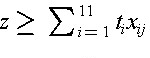
In the previous example, suppose that a mathematical model and solution was desired. For this purpose, we define a binary (i.e. 0 or 1 valued) decision variable for each pipe section and crew, xij, where xij = 1 implies that section i was assigned to crew j and xij = 0 implied that section i was not assigned to crew j. The time required to complete each section is ti. The overall time to complete the nine sections is denoted z. In this case, the problem of minimizing overall completion time is:

subject to the constraints:
xij is 0 or 1
where the constraints simply insure that each section is assigned to one and only one crew. A modification permits a more conventional mathematical formulation, resulting in a generalized bottleneck assignment problem:
Minimize z
subject to the constraints:
xij is 0 or 1
This problem can be solved as an integer programming problem, although at considerable computational expense. A common extension to this problem would occur with differential productivities for each crew, so that the time to complete an activity, tij, would be defined for each crew. Another modification to this problem would substitute a cost factor, cj, for the time factor, tj, and attempt to minimize overall costs rather than completion time.
10.9 Scheduling with Resource Constraints and Precedences
The previous section outlined resource oriented approaches to the scheduling problem. In this section, we shall review some general approaches to integrating both concerns in scheduling.
Two problems arise in developing a resource constrained project schedule. First, it is not necessarily the case that a critical path schedule is feasible. Because one or more resources might be needed by numerous activities, it can easily be the case that the shortest project duration identified by the critical path scheduling calculation is impossible. The difficulty arises because critical path scheduling assumes that no resource availability problems or bottlenecks will arise. Finding a feasible or possible schedule is the first problem in resource constrained scheduling. Of course, there may be a numerous possible schedules which conform with time and resource constraints. As a second problem, it is also desirable to determine schedules which have low costs or, ideally, the lowest cost.
Numerous heuristic methods have been suggested for resource constrained scheduling. Many begin from critical path schedules which are modified in light of the resource constraints. Others begin in the opposite fashion by introducing resource constraints and then imposing precedence constraints on the activities. Still others begin with a ranking or classification of activities into priority groups for special attention in scheduling. One type of heuristic may be better than another for different types of problems. Certainly, projects in which only an occasional resource constraint exists might be best scheduled starting from a critical path schedule. At the other extreme, projects with numerous important resource constraints might be best scheduled by considering critical resources first. A mixed approach would be to proceed simultaneously considering precedence and resource constraints.
A simple modification to critical path scheduling has been shown to be effective for a number of scheduling problems and is simple to implement. For this heuristic procedure, critical path scheduling is applied initially. The result is the familiar set of possible early and late start times for each activity. Scheduling each activity to begin at its earliest possible start time may result in more than one activity requiring a particular resource at the same time. Hence, the initial schedule may not be feasible. The heuristic proceeds by identifying cases in which activities compete for a resource and selecting one activity to proceed. The start time of other activities are then shifted later in time. A simple rule for choosing which activity has priority is to select the activity with the earliest CPM late start time (calculated as LS(i,j) = L(j)-Dij) among those activities which are both feasible (in that all their precedence requirements are satisfied) and competing for the resource. This decision rule is applied from the start of the project until the end for each type of resource in turn.
The order in which resources are considered in this scheduling process may influence the ultimate schedule. A good heuristic to employ in deciding the order in which resources are to be considered is to consider more important resources first. More important resources are those that have high costs or that are likely to represent an important bottleneck for project completion. Once important resources are scheduled, other resource allocations tend to be much easier. The resulting scheduling procedure is described in Table 10-14.
The late start time heuristic described in Table 10-14 is only one of many possible scheduling rules. It has the advantage of giving priority to activities which must start sooner to finish the project on time. However, it is myopic in that it doesn't consider trade-offs among resource types nor the changes in the late start time that will be occurring as activities are shifted later in time. More complicated rules can be devised to incorporate broader knowledge of the project schedule. These complicated rules require greater computational effort and may or may not result in scheduling improvements in the end.
TABLE 10-14 A Resource-Oriented Scheduling Procedure
Example 10-9: Resource constrained scheduling with nine activities.
As an example of resource constrained scheduling, we shall re-examine the nine activity project discussed in Section 10.3. To begin with, suppose that four workers and two pieces of equipment such as backhoes are available for the project. The required resources for each of the nine project activities are summarized in Table 10-15. Graphs of resource requirements over the 30 day project duration are shown in Figure 10-17. Equipment availability in this schedule is not a problem. However, on two occasions, more than the four available workers are scheduled for work. Thus, the existing project schedule is infeasible and should be altered.
TABLE 10-15 Resources Required and Starting Times for a Nine Activity Project
Figure 10-17 Resources Required over Time for Nine Activity Project: Schedule I
The first resource problem occurs on day 21 when activity F is underway and activities G and H are scheduled to start. Applying the latest start time heuristic to decide which activity should start, the manager should re-schedule activity H since it has a later value of LS(i,j), i.e., day 25 versus day 22 as seen in Table 10-15. Two workers become available on day 23 after the completion of activity G. Since activity H is the only activity which is feasible at that time, it is scheduled to begin. Two workers also become available on day 24 at the completion of activity F. At this point, activity I is available for starting. If possible, it would be scheduled to begin with only two workers until the completion of activity H on day 28. If all 4 workers were definitely required, then activity I would be scheduled to begin on day 28. In this latter case, the project duration would be 34 days, representing a 4 day increase due to the limited number of workers available.
Example 10-10: Additional resource constraints.
As another example, suppose that only one piece of equipment was available for the project. As seen in Figure 10-17, the original schedule would have to be significantly modified in this case. Application of the resource constrained scheduling heuristic proceeds as follows as applied to the original project schedule:
- On day 4, activities D and C are both scheduled to begin. Since activity D has a larger value of late start time, it should be re-scheduled.
- On day 12, activities D and E are available for starting. Again based on a later value of late start time (15 versus 13), activity D is deferred.
- On day 21, activity E is completed. At this point, activity D is the only feasible activity and it is scheduled for starting.
- On day 28, the planner can start either activity G or activity H. Based on the later start time heuristic, activity G is chosen to start.
- On completion of activity G at day 30, activity H is scheduled to begin.
The resulting profile of resource use is shown in Figure 10-18. Note that activities F and I were not considered in applying the heuristic since these activities did not require the special equipment being considered. In the figure, activity I is scheduled after the completion of activity H due to the requirement of 4 workers for this activity. As a result, the project duration has increased to 41 days. During much of this time, all four workers are not assigned to an activity. At this point, a prudent planner would consider whether or not it would be cost effective to obtain an additional piece of equipment for the project.
Figure 10-18 Resources Required over Time for Nine Activity Project: Schedule II
10.10 References
- Au, T. Introduction to Systems Engineering--Deterministic Models, Addison-Wesley, Reading, MA, 1973, Chapter 8.
- Baker, K., An Introduction to Sequencing and Scheduling, John Wiley, 1974.
- Jackson, M.J., Computers in Construction Planning and Control, Allen & Unwin, 1986.
- Moder, J., C. Phillips and E. Davis, Project Management with CPM, PERT and Precedence Diagramming, Van Nostrand Reinhold Company, Third Edition,1983.
- Willis, E. M., Scheduling Construction Projects, John Wiley & Sons, 1986.
|
